A remark on the balls hidden inside HDBSCAN
Density based clustering aims at defining clusters where the points are most packed, and separates these clusters by regions where points are sparse. To do this, a density based clustering algorithm has to estimate how “packed” a region is, locally. In this note, the focus is on the way the HDBSCAN algorithm does this, in dimension 2.
In some use cases of density based clustering, we may be looking for long, thin, string shaped clusters, for instance if we are trying to detect cracks in an image, faults from the locations of earthquakes, or filaments in a map of galaxies. The question I asked myself is whether the way HDBSCAN [1] estimates local “packedness” is adapted to these types of clusters ?
Clearly, the simple Single Linkage algorithm is very adapted to finding string-shaped clusters, but it is precisely its sensitivity to these types of shapes (which may be pure noise) that motivates the use of HDBSCAN instead. Is it possible to get the best of both worlds ?
How does HDBSCAN estimate local “packedness” ?
The statistical setting the following. We look at \(X_1,\ldots,X_n\), independent observations from a probability distribution \(P\) on \(\mathbb R^2\). Given a hyper parameter \(k\), HDBSCAN defines, for any point \(x\), the radius \(r_k(x)\), which is the distance from \(x\) to its \(k\)-th closest neighbor among the observations
\[r_k(x) := \inf \{ r>0, \ \# B(x,r)\cap\{X_1,\dots,X_n \}\geq k \}.\]The HDBSCAN intuition is that if \(r_k(x)\) is small, \(x\) has to be in a high density, packed region. More mathematically, the ball \(B(x, r_k(x))\) contains \(k\) of the \(n\) observations, so its mass is \(k/n\), spread over the area \(\pi r_k(x)^2\). This directly gives one way to estimate local packedness, which corresponds to the classical \(k\)-nearest-neighbour density estimate:
\[\hat f_k(x) = \frac{k}{n\,\pi\, r_k(x)^2}. \tag{1}\]The simplest way to understand how HDBSCAN works is to start from Single Linkage. In Single Linkage, we make a threshold \(t\) grow from \(0\), and we join two observations in a representation graph as soon as their distance is at most \(t\). The clusters are then defined as the connected components of the thus defined representation graph of the observations. As the threshold \(t\) increases, the groups merge, and this gives a hierarchy of clusters. HDBSCAN does the same, but it only connects two observations if they are in a “sufficiently packed” region. This is done by replacing the traditional distance between observations used by Single Linkage by the following quantity
\[d_{\text{reach}}(a,b) = \max\big(r_k(a),\, r_k(b),\, \|a-b\|\big).\]To sum it up, Single Linkage asks for two observations to be close to connect them in its representation graph. And HDBSCAN additionally asks that the two observations lie in a packed region: \(r_k(a)\) and \(r_k(b)\) have to be small enough as well for the edge between \(a\) and \(b\) to exist in the graph. Thus, the noise points, which usually lie in sparse regions (and hence have large \(r_k\)), are much harder to connect, and they can no longer easily glue two clusters together.
So in HDBSCAN, the “packedness” around an observation \(x\) is estimated through one single number, the radius \(r_k(x)\) of the smallest ball centred at \(x\) that holds \(k\) observations. The question is: what does this ball see when the clusters we are looking for are string-shaped ?
What a ball sees on a string
We look at the case where an observation \(x\), represented by the star on the plot below, lies in a thin band of observations. Its \(k = 8\) nearest neighbours among the other observations are drawn in blue, and we also draw the ball \(B(x, r_8(x))\) that HDBSCAN uses to measure how “packed” the region around \(x\) is.
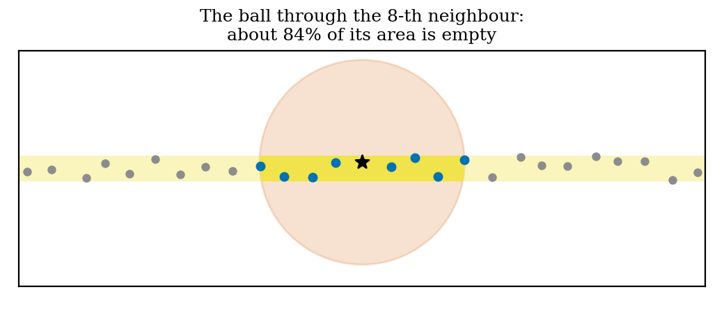
Most of the ball actually ends up being empty in this case. The neighbours all lie only in the yellow band. The estimate in (1) divides the mass contained in this thin band by the area of the whole ball, which is too large. We end up with a bad estimation of the local density and thus of the local packedness.
Let’s try to assess actually how wrong this estimation is. Consider some observations spaced \(\delta\) apart along a straight band of width \(w\), with \(w\) small compared with \(k\delta\). Then, the \(k\) nearest neighbours of an observation sit about \(k/2\) on each side, so \(r_k \approx k\delta/2\) and (1) gives
\[\hat f_k \approx \frac{k}{n\,\pi\,(k\delta/2)^2} = \frac{4}{n\,\pi\,k\,\delta^2}.\]But inside the band, the truth is that there is about one observation per area \(\delta w\), which gives a density \(f \approx 1/(n\,\delta\, w)\). Hence
\[\frac{f}{\hat f_k} \approx \frac{\pi\, k\,\delta}{4\,w}.\]In the case of the picture, we have \(k=8\) and \(\delta = w = 0.12\), so the ratio in that case is equal to about \(6\), which means that the HDBSCAN estimate is quite wrong. What we can takeaway from this is the two following remarks.
- On a thin band of observations, increasing \(k\) makes things worse. Taking more neighbours is the usual way to reduce variance, but in this case it would not work. The bias factor grows as \(k\): the more neighbours we use, the sparser every thin structure looks, whatever its true width really is.
- On a thin band, the ball overreacts to how densely the band is sampled. If the observations are twice as close to each other along the band, the band is twice as dense. But the ball around each observation becomes twice as small in every direction, so its area is divided by four, and (1) becomes four times larger.
This does not mean that estimating packedness with a ball shape is a mistake as such. It means that on thin, string shaped structures, it is probably not the best choice we can make.
Why an ellipse would be better
Even if not ideal, an ellipse fitted to the shape defined by the \(k\) nearest neighbours would already do better than the ball at estimating the actual “string shaped packedness”. Let’s look at the empirical covariance matrix \(\Sigma\) of the \(k\) neighbours of a point \(x\): its eigenvectors give the orientation of the neighbourhood, and its eigenvalues indicate how spread it is along each eigendirection.
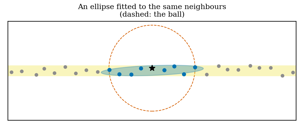
Let’s redo the computation of the previous section, but this time with an ellipse instead of the HDBSCAN ball. For the sake of simple computations and intuition, consider the case where the \(k\) neighbours are spread uniformly over a piece of band of length \(L\) and width \(w\). The ellipse fitted to them then simply spans this piece of band: its axes point along and across the band, with half-lengths \(L/2\) and \(w/2\). Its area is
\[\pi \cdot \frac{L}{2} \cdot \frac{w}{2} = \frac{\pi}{4}\, L\, w ,\]which is now proportional to the area \(Lw\) that the neighbours actually occupy, instead of including all the empty space around them. If we put this area in place of the area \(\pi r_k^2\) of the ball in (1), with \(L \approx k\delta\), we get an estimate proportional to \(1/(\delta w)\), which corresponds to the true density of the band up to a constant. Hence the bias we found for the ball is gone. This remark exists in the literature; for instance, [3] starts by estimating a density with the area of the local covariance ellipse rather than the area of a ball.
The problem: a “noise bridge” is a string too
Back to the question of the introduction; HDBSCAN is generally preferred to Single Linkage precisely because we don’t want thin lines of noise to glue clusters together. Unfortunately, such a line of noise looks like a string like any other, and the computation above applies to it as well.
Take two clouds of observations joined by a thin bridge of noise, as in the figure below. Seen through a ball, the observations of the bridge lie in a sparse region, and HDBSCAN keeps the two blobs apart. But seen through a fitted ellipse, the bridge looks almost as packed as the blobs themselves… A density based method then has every reason to merge the two blobs, and this is what happens when we replace the area of the ball by the area of the ellipse in (1): in one of our three runs the blobs get merged (on the right below), and on average the ARI drops from 0.96 to 0.80.
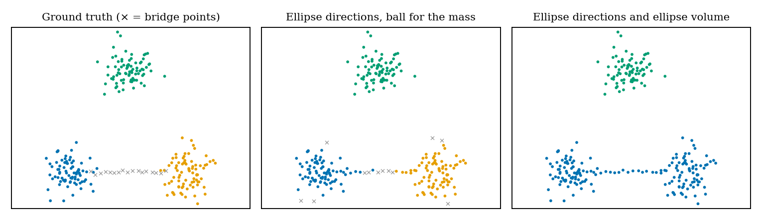
In conclusion, simply replacing the balls in HDBSCAN by ellipses reintroduces one of the biases this algorithm was built to avoid. To get the best of both worlds, the two approaches have to be combined.
Ball for the mass, ellipse for the direction
What the ellipse sees and the ball does not is the direction of the string. So we try keeping the ball for local mass estimating, and we use the ellipse only for the orientation information it gives. To do so, we keep the shape of the ellipse but not its size: we rescale the covariance matrix so that its determinant is \(1\), as
\[A_x = \frac{\tilde\Sigma_x}{\sqrt{\det \tilde\Sigma_x}},\]where \(\tilde\Sigma_x\) is the covariance matrix of the neighbours, slightly mixed with the identity so that the ellipse does not become infinitely thin when the neighbours are almost aligned (we use \(\tilde\Sigma_x = 0.7\,\Sigma_x + 0.3\,\tfrac{\operatorname{tr}\Sigma_x}{2}\, I\)). We then measure distances from \(x\) with this shape, \(\delta_x(y) = \sqrt{(y-x)^\top A_x^{-1}(y-x)}\). Because \(\det A_x = 1\), the region defined by \(\{\delta_x \le t\}\) is an ellipse, with exactly the same area as the disc of radius \(t\). This region is stretched along the string and squeezed across it, but it is neither larger nor smaller than the ball. Hence, the size of the neighbourhoods is still estimated by the “HDBSCAN balls”, and only their orientation changes. Note that elliptical neighbourhoods with the same area as the disc are the idea behind ADCN [4], an anisotropic variant of DBSCAN. And deciding connections from locally estimated principal directions goes back at least to correlation clustering methods such as 4C [5]. Here they are simply used to enrich the classical mutual reachability distance, which becomes
\[d(a,b) = \max\big(r_k(a),\, r_k(b),\, \delta_a(b),\, \delta_b(a)\big),\]so that two observations are connected at threshold \(t\) in the representation graph when both the \(r_k\) are below \(t\) and each lies inside the other’s neighbourhood of size \(t\), now oriented along the local structure.
But when does the direction actually change anything ? Between two close neighbours on a string, \(\|a-b\|\approx\delta\) is much smaller than \(r_k\approx k\delta/2\), so the maximum is reached by the core distances and the direction plays no role at all. It only matters when the distance term is the bottleneck, that is when there is a gap in the string. Meaning when two consecutive observations \(a\) and \(b\) of the string are separated by an empty stretch of length \(g = \|a-b\|\), larger than the radiuses \(r_k(a)\) and \(r_k(b)\). Let \(e\) denote the largest eigenvalue of \(A_x\). Since \(\det A_x = 1\), the other eigenvalue is \(1/e\), so that, measured with \(\delta_x\), a distance along the string is divided by \(\sqrt e\) while a distance across the string is multiplied by \(\sqrt e\). If the ellipses of \(a\) and \(b\) are both aligned with the string, \(a\) and \(b\) get connected in the representation graph at threshold
\[\max\big(r_k(a),\, r_k(b),\, g/\sqrt e\big) \quad\text{instead of}\quad \max\big(r_k(a),\, r_k(b),\, g\big)\]with the ball, so the gap stops cutting the string in two earlier. On the other hand, two observations lying on two parallel strings at distance \(h\) from each other get connected at threshold \(\max\big(r_k(a),\, r_k(b),\, h\sqrt e\big)\) instead of \(\max\big(r_k(a),\, r_k(b),\, h\big)\). The ellipse fills holes along a string and delays connections between neighbouring strings, at no cost in mass.
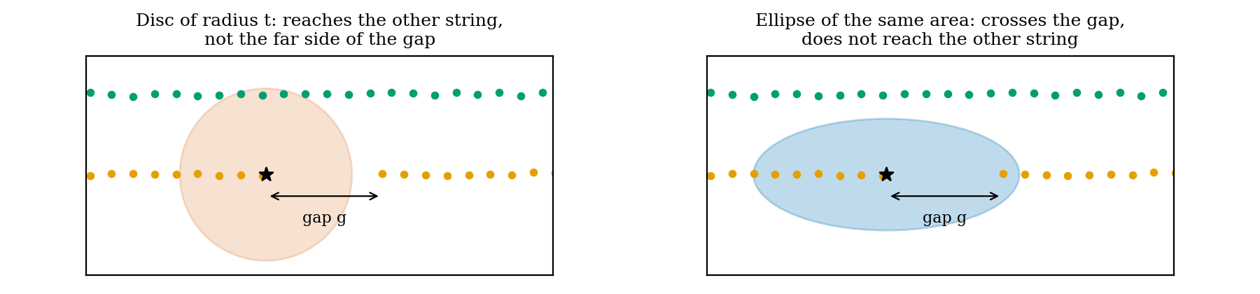
This helps precisely in the case of “string-shaped” structures sampled at random positions, like the sinusoids below. Note that the regularisation on the local covariance caps the effect of the ellipses (this is intented): for perfectly aligned neighbours, \(\tilde\Sigma_x\) has eigenvalues in the ratio \(0.85 : 0.15\), which gives \(e \approx 2.38\), so gaps can only be at most about \(\sqrt e \approx 1.5\) times longer than with the ball. But of course, this also tells where this approach will hurt: with a bridge whose gaps are short enough connects the two clusters earlier, for the same reason.
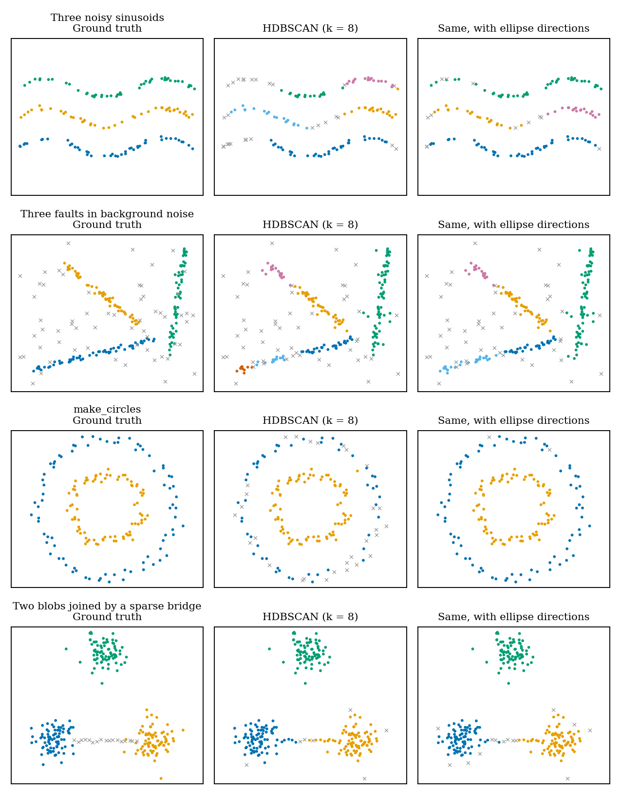
On a few synthetic configurations of dimension \(2\) string shaped clusters, (with ARI on the points that are not noise, averaged over three random draws; the number of clusters is given to neither method), this gives:
| HDBSCAN, \(k=8\) | with ellipse directions, \(k=8\) | HDBSCAN, best \(k\) | with directions, best \(k\) | |
|---|---|---|---|---|
| three noisy sinusoids | 0.66 | 0.86 | 0.75 | 0.95 |
| three faults in background noise | 0.62 | 0.77 | 0.62 | 0.77 |
| three lines of different sampling density | 0.81 | 0.96 | 0.87 | 0.99 |
| two concentric circles | 0.70 | 0.99 | 1.00 | 1.00 |
| two blobs and a sparse bridge | 0.96 | 0.96 | 0.99 | 0.99 |
| two blobs and a dense bridge | 0.79 | 0.57 | 0.79 | 0.70 |
The comparison at a fixed \(k\) flatters the change: on the circles, HDBSCAN with \(k=5\) is already perfect, and the gain at \(k=8\) only reflects a poor choice of \(k\). On the sinusoids, the faults and the lines, the gain survives when each method gets its best \(k\). The sparse bridge is left untouched, which is the point of keeping the ball for the mass. On the dense bridge though, the result gets worse, as expected. When the noise bridge actually is a dense line, directions make it easier to follow, like any other actual cluster string. And “following strings” also means absorbing a bit more of the surrounding noise: on the faults, the share of background points left as noise drops from 0.76 to 0.69.
So, the best of both worlds ? Partly. With the mass measured by the ball and the direction by the ellipse, HDBSCAN follows strings much better without letting sparse bridges through. What no local shape can do is tell a dense noise bridge apart from a legitimate string. This happens precisely because locally, the two look are the same object, and only the amount of mass around them may separate them.
References
[1] R. J. G. B. Campello, D. Moulavi, J. Sander. Density-based clustering based on hierarchical density estimates. PAKDD, 2013.
[2] K. Chaudhuri, S. Dasgupta. Rates of convergence for the cluster tree. NeurIPS, 2010.
[3] J. A. Kovacs, C. Helmick, W. Wriggers. A balanced approach to adaptive probability density estimation. Frontiers in Molecular Biosciences 4:25, 2017.
[4] G. Mai, K. Janowicz, Y. Hu, S. Gao. ADCN: an anisotropic density-based clustering algorithm for discovering spatial point patterns with noise. Transactions in GIS, 2018.
[5] C. Böhm, K. Kailing, P. Kröger, A. Zimek. Computing clusters of correlation connected objects. SIGMOD, 2004.